Excel for SEO Success: Top 10 Formulas Every SEO Needs to Know
Need Excel tips to help with SEO? These are the formulas and functions that SEOs ask us about all the time. Use them to save time and produce better work.
All SEOs need basic Excel skills — whether it’s conducting SEO audits, putting together reports, diving into exported Conductor platform data, or making changes through our Bulk Update feature. Luckily, these frequently asked about Excel for SEO tricks are about to make your life just a little bit easier.
The Top 10 SEO Excel Formulas
- How do I combine the contents of Cell A with Cell B?
- How can I easily change out a folder in a URLURL
The term URL is an acronym for the designation "Uniform Resource Locator".
Learn more when putting together a redirect document? - How can I calculate the length in characters of my Title and Meta Descriptions?
- How do I remove all these extraneous spaces?
- How to a change these keywords to all lowercase?
- How to a change these keywords to all uppercase – they are acronyms?
- How to a format a list of names into propercase that come in as All Caps?
- How can I check to see if a keywordKeyword
A keyword is what users write into a search engine when they want to find something specific.
Learn more in List B is in another list of keywords (List A)? - How can I check to see if a keyword in List B is in another list of keywords (List A) – but information is in rows?
- How do I clean-up #N/A’s from other Excel Formulas?
1. How do I combine the contents of Cell A with Cell B?
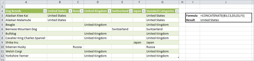
Excel Function: CONCATENATE
Merge text from multiple cells with the formula =CONCATENATE(text1, [text2], …)

This is helpful when you need to:
a) Combine contents of different cells with information.
For example, put the string (or text) in quotes: =CONCATENATE(A1,”, “,A2) will combine the contents of A1 with a comma and space and then display A2.
b) Combine columns for Standard Categories to add to Conductor by Keyword.
c) Perform Keyword Research.
Use Concatenate in keyword research by working with modifiers before or after a set of keywords. For example, if you have the keyword “dog” and attributes such as color “brown” or “white” or “black,” size “large” or “lap” or “under 30 lbs,” or geo location “Park in NYC” or “Vet in San Fran” or “Daycare in Vancouver” – you can make a number of combinations by changing out what is combined:

Note: It is also useful to append Google Analytics parameters to URLs for various marketing campaigns – having a sheet of all the parameters in use can really help you keep track and minimize duplicates due to case sensitivity.
2. How can I easily change out a folder in a URL when putting together a redirect document?
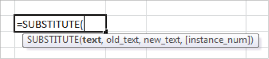
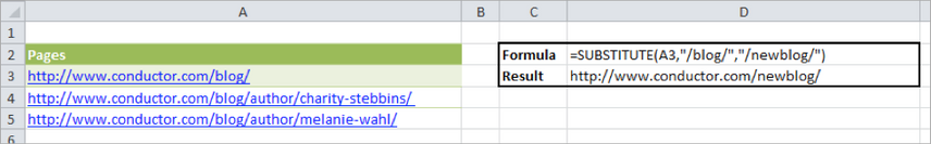
Excel Function: SUBSTITUTE
If you have a list of URLs that are set to be redirected, you can quickly generate the new list using =SUBSTITUTE(text, old_text, new_text, [instance_num])
text: the cell you want to source to make changes based on.
old_text: represents the part of that source material you wish to change.
new_text: what you wish to replace “old_text” with.
[instance_num]: a count in case there are multiple instances of “old_text” for you to replace. For example, if the folder structure is used in part a second time in the URL, it is optional.
This is similar to the actions of Find & Replace, however, it allows for a second list to be generated without saving over the first list.
There are a number of keyword and URL level applications with the SUBSTITUTE Function:
-Given keywords with underscores instead of spaces? Reformat URLs from _ to –
-Switching from .htm to .html or another variation.
-Moving to a Secure Site and need a list of your new pages: http to https.
-Duplicating Clusters of Keywords: Blue-related Keywords to Red-related Keywords? Just Substitute “blue” for “red” and have a whole new keyword list.
3. How can I calculate the length in characters of my Title and Meta Descriptions?
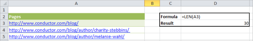
Excel Function: LEN
There comes a time for every SEO to know this formula. =LEN(text) is a simple way to get the Length of a URL, a Title, a Meta DescriptionMeta Description
The meta description is one of a web page’s meta tags. With this meta information, webmasters can briefly sketch out the content and quality of a web page.
Learn more, or an Alt Tag for a large number of cells.
4. How do I remove all these extraneous spaces?
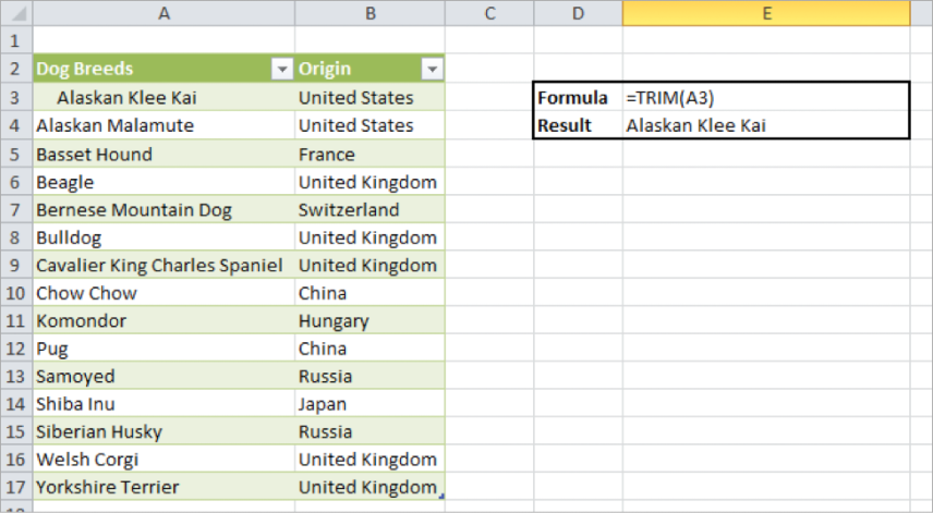
Excel Function: TRIM
Ever collected a large amount of data and found it formatted strangely with lots of extra spaces included? There’s a really easy way to cut out the space you don’t want, but keep the spaces between the words you need. SEO, meet formula: =TRIM(text)
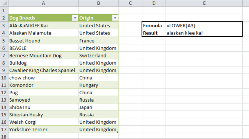
5. How to a change these keywords to all lowercase?
Excel Function: LOWER
Have inconsistent caps for your keywords? =LOWER (text) is a pretty straightforward formula for making everything lowercase.
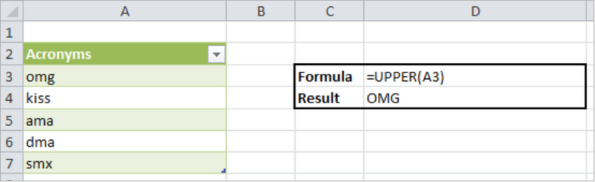
6. How to a change these keywords to all uppercase when they’re acronyms?
Excel Function: UPPER
=UPPER(text) is an easy way to convert H1s to all caps. Another great formula for cleaning up data.
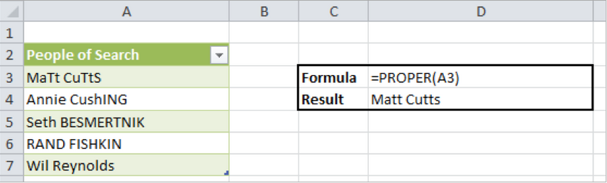
7. How do you format a list of names into proper case that are all caps?
Excel Function: PROPER
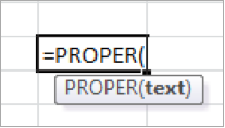
=Proper(text) is an easy way to change a list of names into proper case.
8. How can I check to see if a keyword in List B is in another list of keywords (List A)?
Excel Function: VLOOKUP
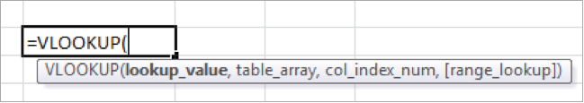
=VLOOKUP(lookup_value, table_array, col_index_num, [range_lookup]) looks for a value in the left column of a table, and then gives you the value in the row from a column you want.
Lookup_value: this is what you want to look for
Table_array: this is where you want to look for it
Col_index_num: this is what you want the formula to return
Range_lookup: if you want an exact match, mark this is FALSE
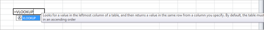
Note: VLOOKUP only works if the data you are looking for is in the first column (the leftmost column) and the data must be in ascending order (A-Z).
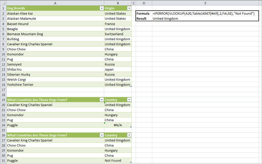
Let’s go to an example. If we look up A20 (Cavalier King Charles Spaniel) in the Dog Breeds table (A1:B16 – named here as Table14567(#All)) using VLOOKUP in cell B20, and are looking to find out its country of origin, we would select 2 for the Col_index_num to look for Origin Country. If Cavalier King Charles Spaniel was not found in the Dog Breeds table the formula would return #N/A.

9. How can I check to see if a keyword in List B is in another list of keywords (List A) – but the information is in rows?
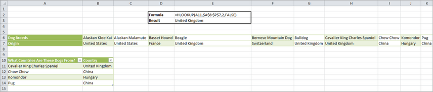
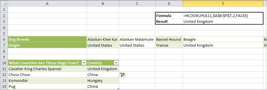
Excel Function: HLOOKUP

=HLOOKUP(lookup_value, table_array, row_index_num, [range_lookup]) is similar to VLOOKUP but with rows rather than columns.
Lookup_value: this is what you want to look for
Table_array: this is where you want to look for it
Row_index_num: this is what you want the formula to return
Range_lookup: if you want an exact match, mark this is FALSE
10. How do I clean-up #N/As from other Excel Formulas?
Excel Function: IFERROR
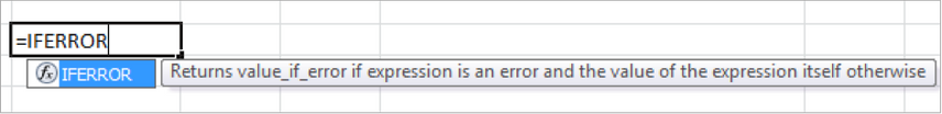
Use =IFERROR around VLOOKUP or HLOOKUP to clean up your data.
Notice in the example that if we add “Puggle” to the list of Dogs are looking up, but it is not in the Dog Breeds table a VLOOKUP formula will return “#N/A” (Cell B24). If we add the IFERROR formula around the VLOOKUP formula with the string “Not Found” to be displayed instead of “#N/A” we see it in Cell B31.